
This page focuses on modeling WW2 battle outcomes in Mathematica.
First there is a raw Excel data file that was the starting point of the analysis, containing rows for various WW2 battles with columns for engaged forces, battle parameters, and various outcomes.
Next there is a prepared data file in a test format meant to be read in as a Mathematica .m file, suitable for working with the processed data in the code notebooks provided and discussed below. It is zipped for attachment to this website and needs to be unzipped to be read properly.
Next there is the main Mathematica code notebook, WW2Analyzed.nb Again this has to be zipped to be attached here, and you will either need a version of Mathematica or to use the Wolfram Cloud to get this to run.
Those are for people interested in following or reproducing all aspects of the analysis, or in using the dataset to work on their own models. Below I present some graphs of the relationships found.
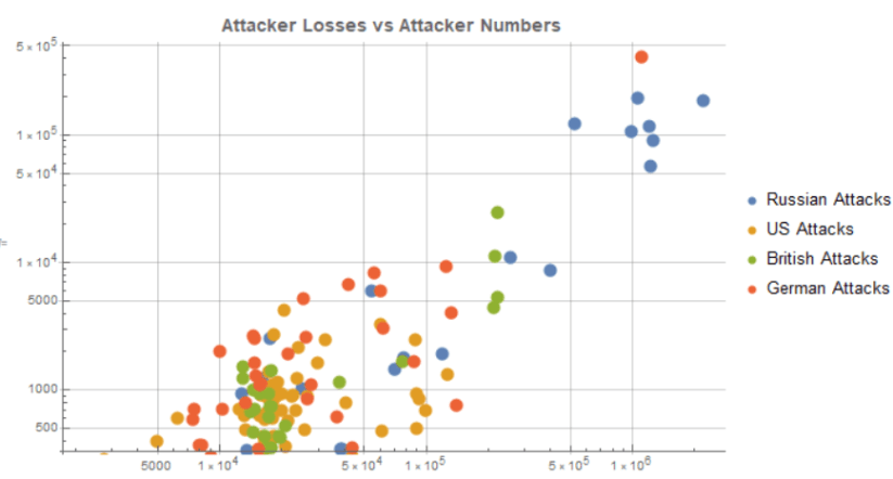
First the primary evidence of log loss scaling is simply to plot each side’s losses against their own numbers across all engagements. That gives the following, for attackers and then defenders –

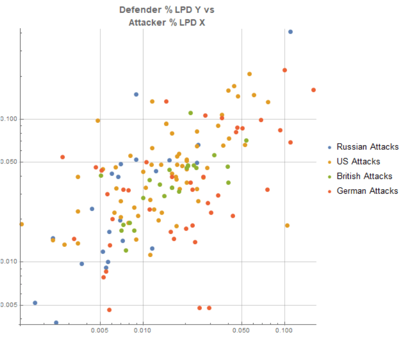
The next relationship of importance is that defender’s losses per day and attacker losses per day are correlated, apparently reflecting a kind of “combat intensity” set by how hard the attacker “pressed” his attacks. We have already incorporated the “own size” information into this and controlled for different battle lengths in time, since now each side’s losses are being expressed as percentages of their engaged forces per day of the combat. This relationship is “noisier” but the correlation is still graphically evident.
A still stronger relationship can now be found between the defender’s loss rate (percent of engaged forces) per day of combat as a function of the attacker’s odds. This (below, next graphic) is already getting us close to what wargame CRTs are trying to model. Notice that the “scatter” around the trend relationship is effectively our “unexplained by odds” residual, which we’d like to tighten using other factors if possible, but will “leave” to the die roll dispersion around the expectation if we cannot reduce it further. The strength of this relationship is an RSquared of 0.56, quite good by “social science standards”. This is the core of what a good operational CRT needs to capture as you move across its columns. Note that both axes are logged and the vertical is percentage of the defending force lost per day of combat, while the horizontal is a raw numerical strength ratio. Later we will improve that to equipment-adjusted combat power measures.
As for the nation breakdowns, while the US attacks give considerably higher enemy percentage losses for a given level of odds and the Germans somewhat higher, and UK attacks somewhat lower, none of the single nation factors reached the threshold of statistical significance. The US effect is closest with a T-stat of 1.77 standard deviations – the orange-yellow points below are “lifted” a bit above the fit line. The US effect would be worth plus 2/3rds of one odds column; the German effect (T-score about half the US one) is worth 1/3rd of one odds column. The odds ratio itself is significant to the tune of 13.3 standard deviations, clearly driving.

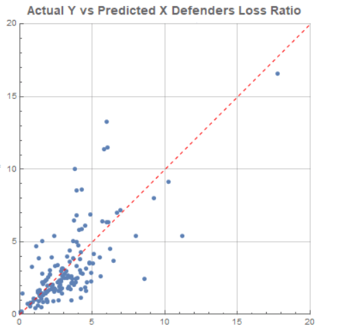
And here is the predicted vs actual defender loss ratios one gets if one uses that relationship, after dropping the national factors as not at the level of statistical significance. Here the units are percentage losses per day on both axes, with the dispersion around the perfect prediction line X = Y the residual left for chance or other factors to explain.
This is already decent, but we’d like to do better. In addition, we still need to get a prediction for attacker loss rate and probability of an advance rate over some threshold level. For that we are going to need more factors in our model, and many more measures calculated from the raw data in the excel file. These are the columns created for the WW2Analyzed.m data file in the first zip attachment above.
One record in the fully prepared dataset with its extra calculated columns looks like this –
{“Attacker” -> “Russia”, “BattleID” -> 490.,
“AttackerName” -> “SOV Kalinin AG”,
“DefenderName” -> “GER AG Centre”, “AttNum” -> 1.0603*10^6,
“AttTanks” -> 667., “AttGuns” -> 3440., “AttPower” -> 0.648647,
“DefNum” -> 880000., “DefTanks” -> 850., “DefGuns” -> 2050.,
“DefPower” -> 0.622159, “Advance” -> 143., “AttLoss” -> 197591.,
“DefLoss” -> 273866., “Days” -> 34., “Width” -> 1060.,
“Posture” -> “Hasty”, “Terrain” -> “Normal”, “Weather” -> “Normal”,
“Air” -> “None”, “Surprise” -> “Attacker”, “TankRatio” -> 0.784706,
“GunRatio” -> 1.67805, “APLD” -> 0.005481, “DPLD” -> 0.00915328,
“DRelLoss” -> 1.38602, “DRelPLoss” -> 1.67, “DLossPerA” -> 0.258291,
“ALossPerD” -> 0.224535, “DLossPerAD” -> 0.0075968,
“ALossPerDD” -> 0.00660398, “DLossPerAP” -> 0.3982,
“ALossPerDP” -> 0.360897, “DLossPPerAP” -> 4.525*10^-7,
“ALossPPerDP” -> 3.40372*10^-7, “DLossPPerAPD” -> 1.33088*10^-8,
“ALossPPerDPD” -> 1.0011*10^-8, “DFSR” -> 830.189, “DFSP” -> 516.509,
“DFSRE” -> 571.825, “DFSPE” -> 355.766, “OddsR” -> 1.20489,
“OddsP” -> 1.25618, “OddsRE” -> 1.4233, “OddsPE” -> 1.48389,
“ScaleR” -> 6.28787, “ScaleD” -> 7.81935, “AdvD” -> 4.20588,
“Depth” -> 0.134906, “DepthD” -> 0.00396781}
Here is the prediction finding for rates of advance, though the relationship found isn’t great. Scale is clearly important as well as the odds ratio, with larger army scale combats more likely to give higher advance rates per day than the smaller division size cases in the dataset.
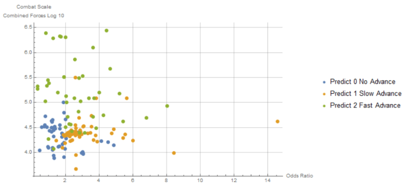
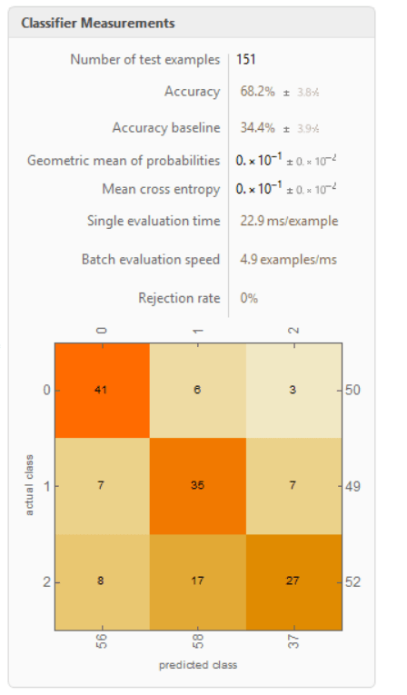
The best classifier found for this gets about 2/3rds of all cases right as to broad advance rate class – none, slow but positive enough to correspond operationally to just winning the defender’s hex, and fast enough to mean DR 2 or removed with a faster advance. That is twice as good as the accuracy of random guessing given the frequencies of these classes. While the actual classifier does more than this, to a first approximation it is saying “if the scale is division or corps size and the odds are below 2-1, there will normally be no advance. If the scale is army size or above and the odds are 3-1 or better, there will be a rapid advance. If the scale is division or corps and the odds are 3-1 or better, there will normally be a small advance”. Here is actual the confusion matrix for this best classifier.
The next question is how much better we can get about the prediction of defender losses if we get to use all our calculated properties, including weapon intensity adjustments to raw numbers – created by awarding 60 power points for each tank and 80 for each gun, on top of 1 point per man, then normalizing for the average weapon intensity across the data which is about 50-50 equipment and personal with those figures – force to space ratios, coded defender stance, air support, and the like.
The set of factors that survived variable elimination for this wound up being –
{“Attacker”, “Posture”, “Terrain”, “Weather”, “Air”, “Surprise”,
“TankRatio”, “DFSP”, “OddsP”, “ScaleR”}
Where attacker means which nation is attacking, posture is how prepared the defense was, terrain is discretized to a few classes, weather is just good enough to allow air or not, air is which side had air superiority if either, surprise is a flag for attacker surprise only set in only a small portion of cases, tank ratio is the armor odds aka attacker tanks (only) divided by defender tanks, DFSP is the defender’s force to space measured in units of intensity adjusted combat power, oddsP is the combat odds measured the same way, and scaleR is the size of the combat as log10 of attacker plus defender numbers, both those in raw personnel terms.
In addition, we can pick a better target to try to predict – the ratio of the percentage losses of the defender divided by the percentage losses of the attacker (note that “per day” drops out of that relationship as the same for both sides). The best method for this winds up being a Gradient Boosted Tree machine learning method, and this is the prediction vs actual relationship it can find.

This time the raw units of the predictions are how many times larger the percentage losses of the defender will be than the percentage losses of the attackers, who will of course generally outnumber the defenders, so their absolute losses are higher for a given loss rate percentage. We see lots of relatively even combats for which this actual ratio lines up quite well with its predicted value while being on the order 1-5 times the attacker’s loss rate, another smaller portion with a bit wider dispersion with relative loss rates in the 5-10 range, and only a few cases outside that range.
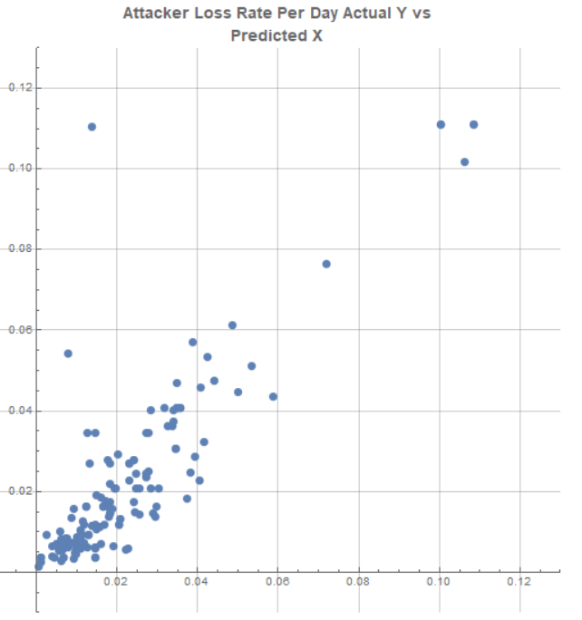
To make full use of that strong relationship, however, we also need to predict how much the attackers will lose in absolute percentage loss per day terms for given conditions of combat. If we can do so, then the above relationship will tell us how to turn those loss expectations into how much higher defender loss rates.
The interesting thing is that attacker loss rates per day don’t follow a normal distribution. Instead they look like this –

These are following a Gamma distribution with fit parameters
FindDistributionParameters[mylosses, GammaDistribution[a, b]]
{a -> 1.31628, b -> 0.0175489}
So instead of trying to predict the raw attacker percentage losses, we want to predict the Z score of attacker losses as a position in that distribution.
We then train a Gradient Boosted Tree model to predict that Z score for each combat. After getting the predicted Z score of losses, transform back to the predicted percentage loss rate. This let’s us find the following full prediction method relationship, end to end, for attacker losses –
Since the whole procedure uses GBT models, I probed the sensitivity of the model to its various factors, and also looked at the linear relationship strengths and p-values of all the input factors vs the outcomes at each stage. Odds, the armor ratio, surprise code, and Russian attackers (a proxy for lower unit quality in this dataset) all mattered, with scale and defender posture mattering much less than one might expect.
As a result of this analysis, I decided that armor odds and unit quality were the most important combat modifiers to keep for both my New SCS and my News OCS combat systems, and that it was worthwhile to keep a Surprise mechanic, though I revised it extensively and toned down both it and quality compared to original OCS.
The scale of the residuals left by this fitting process also determined the dispersion I wanted to keep between “good and bad rolls” on the 2D6 CRTs used for both of those systems. The standard deviation of the fit residuals worked out to about plus or minus how much the expectation moves in one odds column, but in a relationship with significantly higher kurtosis (longer tails) than a normal distribution. Here is what a SmoothKernelDistribution over the empirical fit residuals looks like.

The kurtosis of that shape is 10.37, vs 3 for a normal distribution. On the above plot, points at plus or minus 1.6 are an “odds column” higher or lower than expectation for the power odds, points at plus or minus about 3.2 are “2 odds columns” off the expectation. The probability “weight” in the latter (up or down an amount “worth 2 odds columns”) is about what you expect for rolling 2 or 12 on a 2D6 table. So, really poor rolls or really good rolls should have bad results even at higher columns, and good results even at low columns, respectively, to capture that empirical variance.
I realize that is a lot to follow. I hope it helps to understand the amount of work needed to find proper historical relationships and to encode them into new CRTs like those used in my new SCS and new OCS systems.
